Excel Drop Down Menu - Best Practices in creating a drop down menu in Excel
SHARE
How to create a drop down menu in Excel
-
Select the cell(s) to insert the drop down menu First, select the cell(s) that you want to insert in the drop down menu. This can be one cell, a few cells located apart from each other or a range of cells.
-
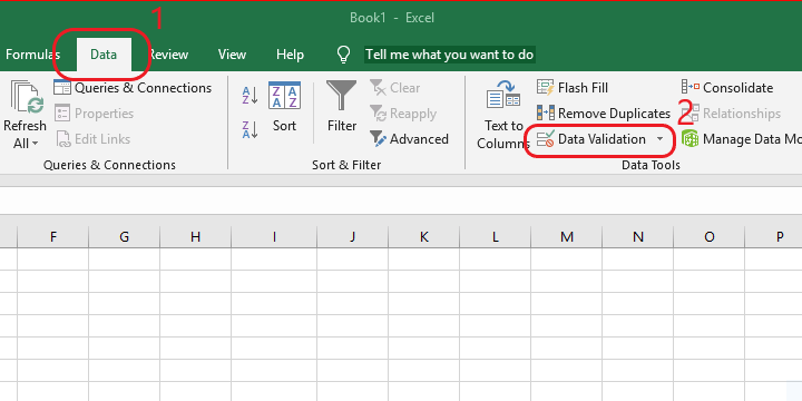
Open the Data Validation dialog box On the Excel ribbon, Go to the “Data” tab → Data Tools → Click “Data Validation”.
-
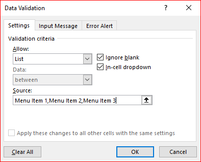
Select “List” from the validation criteria “Allow:” menu Select “List” from the “Allow:” drop down menu in the settings tab of the data validation dialog box.
-
Define the menu items for the drop down menu Method 01: Type the list of menu items within the “Source” input box, each item separated by a comma.
Method 02: Alternatively, you can select a cell range for the source that contains the list of menu items.
-
Apply other relevant settings Tick the “Ignore blank” check box and “In-cell dropdown” check box
-
Apply optional settings for drop down menu Setup “Input message” or “Error Alert” if you need by using relevant tabs in “Data Validation” dialog box.
-
Close the Dialog box Click “OK” to apply the created dropdown menu to the cells.
In Microsoft Excel, it is possible to add a drop down menu to select inputs to a cell from a predefined list by using data validation feature. In our Soccer Prediction App tutorial we created a drop down menu. So if you want you can download the excel file to see a practical example.
There are primarily two types of drop down menu s in Excel.
- Static Dropdown menu – Create a drop down menu by typing a validation list
- Dynamic Dropdown menu – Create a drop down menu by choosing a cell range for menu items
How to create a drop down menu by typing a validation list (Static dropdown menu)
This is the simplest way to add a drop down menu. What you have to do is select the cells in which you want to add a drop down menu in excel. And then,
Go to “Data” tab → Data Tools → Data Validation
Now you will be presented with the “Data Validation” dialog box.
In the “Settings” tab of the Data validation dialog box, select “List” from “Allow” drop down menu.
In the “Source” Input box, type the list of drop down items that you wish to include in your drop down menu.You have to separate each item by a comma. Then make sure that both of the “Ignore Blank” and “In-cell dropdown” check boxes are ticked.
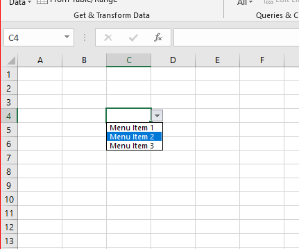
Finally, Click okay and select a cell in which you have inserted the drop down menu. You should see a small down arrow to the right of the cell. Click that small down arrow to find out the drop down menu in excel you just created.
How to create a drop down menu by choosing a cell range for menu items (Dynamic dropdown menu)
In a dynamic drop menu in excel, menu items are typed in a range of cells instead of hard coding inside the “Data Validation” dialog box.
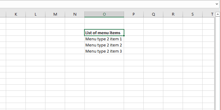
Step 01 : Create a List of menu items in a cell range
Type the list of menu items you would like to have in your drop down menu in excel cell range, one for each cell without keeping empty cells.
You can enter your menu items in a column or row, but it is highly recommended to make your list in a column if you wish to change and update your menu later.
Step 02 : Convert the cell range into a table (Optional but recommended)
This step is optional, but if you convert your cell range into a table you can remove or add menu items by simply adding or removing rows from the table range.
What you have to do is select the cell range having your menu items list, and click the “Insert” in the main menu. Then go to “Tables” command group and click “Table”.
Go to → Insert → Table
Now the “Create Table” dialog box will pop up.
Tick the check box “My table has headers” if your table’s first row is the header. Click OK.
Step 03: Insert the drop down menu into selected cells
Select the cells in which you wish to insert your drop down menu in excel. It can be one cell, a range of cells or few cells which located apart from each other. Now same as previously,
Go to “Data” tab → Data Tools → Data Validation
Select “List” from the “Allow” drop down menu.
Then click the Range selection button at the right edge of the “Source” input box. Now select the range of cells in which your list of menu items is entered. As you did previously, tick both the “Ignore Blank” and “In-cell drop-down” check boxes. Click OK to finish. You will see that drop down menus are active in the cells you have chosen.
Modifying the drop down menu in excel.
There are two methods to modify the drop down menu in excel, depending on the type of drop down menu.
Static drop down menu.
- Select a cell that contains a drop-down menu.
- Go to → “Data” tab → Data Tools → Data Validation
- “Data Validation” dialog box will pop up and you will see the list of menu items you previously entered in the “Source” input box.
- Modify the list of menu items as you wish.
- Tick the relevant check box to apply the changes to all other cells in the worksheet having similar drop-down menus.
- Click OK.
Dynamic drop down menu.
In these types of drop down menus, we use the cell ranges in the work sheet to feed the drop down items list. Therefore, modification of the drop down menu in excel can be done in two ways.
- Change range of cells of source
- Modify the list items within the source cell range.
Changing the range of cells of source
- Select a cell that contains a drop-down menu.
- Go to “Data” tab → Data Tools → Data Validation
- “Data Validation” dialog box will pop up and you will see the previously selected cell range in the source input box.
- Click the Range selection button at the right edge of the “Source” input box and select the new cell range which contains new list of menu items.
- Tick the relevant check box to apply the changes to all other cells in the worksheet having similar drop-down menus.
- Click OK.
Modify the list items within the already selected source cell range.
Following procedure works only if you have converted the cell range you used have already been converted to a table as recommended above.
Add a new menu item to the end of the list:
Type the new menu item just below the last item of the table.
Delete menu items from the list:
- Select the cells that contain menu items you need to remove.
- Right click on a selected cell.
- Go to Delete Table Rows in the appeared pop up menu.
If you only delete the cell content by pressing “backspace” or “delete” key in keyboard, it will show a blank menu item.
How to remove drop down list in excel?
In above section we learned how to add a drop down menu or drop down list in to excel cells. Now let us see how to remove a drop down list in excel cells. You can remove the drop down list in excel cells very easily by following the steps given below.
- Select the cells that you want to remove the drop down list
- Go to → “Data” tab → Data Tools → Data Validation
Now if you have similar and identical drop down lists in each selected cells, it will pop up the Data Validation dialog box when you click the “Data Validation” command button. Otherwise it shows the following message box telling that it has more than one type of data validation and ask to continue with erasing the current settings.

Just click “OK” to confirm and then the Data Validation dialog box will pop up.
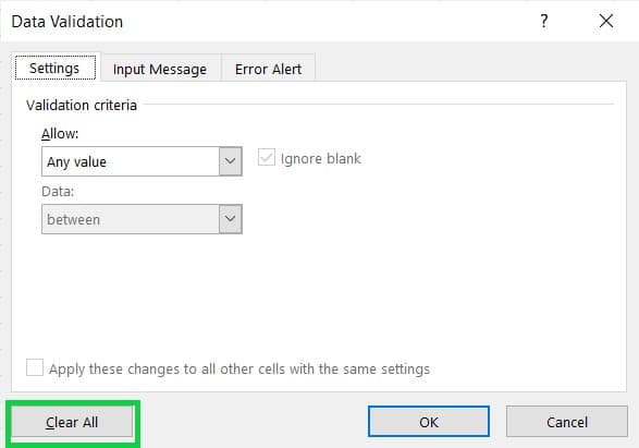
- Click the “Clear All” button in the “Data Validation” dialog box.
- Finally click “OK” to close the data validation dialog box. Now all the drop down menus from the selected cells should be removed.
References:
SHARE