Learn how to use VLOOKUP function

VLOOKUP function can be used to lookup and retrieve data from a given column referenced by a value of the first column.The data set should have been arranged in columns to make it possible to work this function.

Following example of finding the price and stock count of a product referenced by the given product id is a real world example of a situation where we can use VLOOKUP function.

Let us consider a scenario where you need to get the unit price or the available quantity for a given product. What would happen normally is that your eye scans through the first column, where the Product IDs are located to find in which row, the given product id is located. Then the eye move across the identified row to lookup and retrieve relevant unit price or available quantity.

We can automate the same data lookup procedure using Microsoft Excel VLOOKUP function.

Let us follow the simple steps given below to learn how to use the VLOOKUP function.

Step 01: Setting up the data set

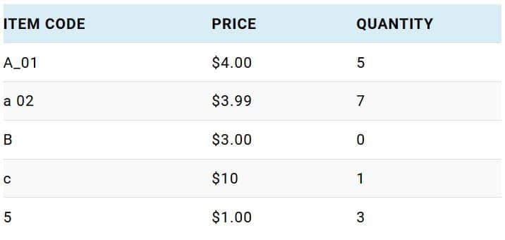
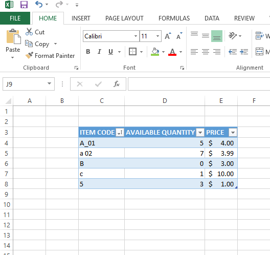
Open Microsoft Excel and create a new Blank workbook. Then enter your data as shown below. I would recommend you to download the free excel file which is all set for you to begin with.

Then choose a cell to enter your preferred “ITEM CODE” and another cell to show expected result.

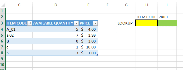
We are going to enter required “ITEM CODE” in cell “H3” and the “PRICE” of the item will show up in “I3”.

Step 02: Calling for VLOOKUP function

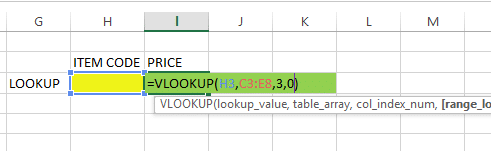
In Cell “I3” type =VLOOKUP(

It shows us some tool-tips that describe the parameters we have to enter within the parentheses.

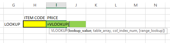
lookup_value : A value in the left most column of the data table,

Here it should be one of the values in “ITEM CODE” column or a reference to it. Since we are going to enter the “ITEM CODE” in cell “H3” , we have to refer cell “H3” for lookup_value, therefore lookup_value parameter should be set to “H3”.

table_array : the range of cells that contains the data to be filtered.

Here it is “C4:E8”

col_index_num : the index number of the column to be filtered out with respect to “lookup_value” counting from left most column.

If you need to filter out price of a given item then this parameter should refer “PRICE” column, which is number three (03).

[range_lookup] : value (TRUE or FALSE) that specifies whether you want VLOOKUP to find an exact match or an approximate match.

I will explain this later, until then, let us set the value to FALSE or value zero (0).

Finally, your function should look like this,

Step 3: LOOKUP for results

Now it is time to see if it works.
Enter one of the values in ITEM CODE column to cell “H3” and see that corresponding price for the specified item appears in cell “I3”.

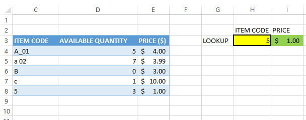
Great! That is what we wanted!

Further if you need to get the available quantity of a given item you just have to modify the col_index_num parameter of the VLOOKUP function.

if you have anything that you do not understand in this tutorial or if you have feedback, feel free to use the comment section below.