How to create a Pivot Table in Excel?
SHARE
In the previous tutorial we learnt what is the pivot table feature in Excel. In this tutorial you will be able to learn how to create a Pivot Table.
Let’s move straight into a simple example. This guide will be very easy and useful for you to understand the essential steps of how to create a pivot table.
Here I am considering a data set containing annual wages of three different ranks of university professors in two different disciplines.
You can download the data set using below link.
In this data set there are columns for id,rank, discipline, years since PHD, years of service, sex and salary. There are exactly 397 rows of data in it.
How to insert the Pivot Table?
How to insert and setting up Pivot Table in Excel
- Step 01
Select any cell within the data set.
- Step 02
Go to “Insert Tab” → “Tables” command group → click “PivotTable”
Create PivotTable dialog box appears.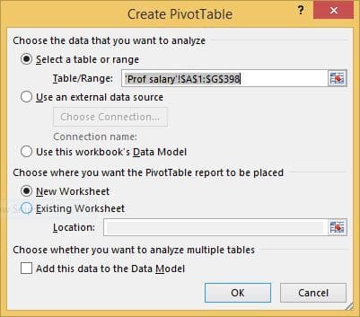
- Step 03
Change the “Table/Range” value to the required cell range where your data set is placed. If the cell range inserted automatically is correct, no need to change anything.
- Step 04
Keep the option “New Worksheet” selected for where you want the PivotTable report to be placed.
- Step 05
Click “OK”
Now, excel creates a dummy Pivot Table in a New Worksheet and displays the Fields Task Pane on the right hand side of the window.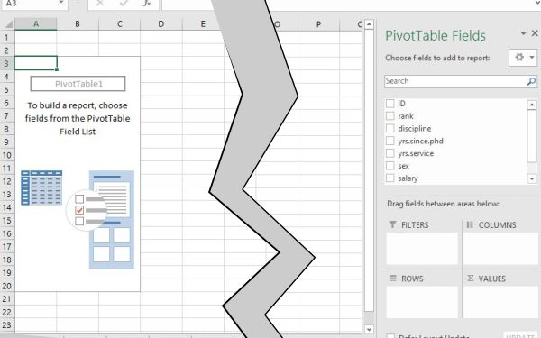
- Step 06
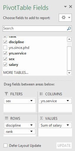
Drag and drop the fields that are needed to be the rows of the Pivot Table into ROWS area. In this example drag the “discipline” and “rank” fields into the ROWS AREA.
- Step 07
Drag and drop the fields that are needed to be the columns of the Pivot Table into COLUMNS area. In this example drag the “yrs.service” field into COLUMNS AREA.
- Step 08
Drag and drop the fields that are needed to use to filter the data in the Pivot Table into FILTER area. Drag and drop “sex” field to FILTER AREA in this example.
- Step 09
Finally drag and drop the fields that should be the values of the Pivot Table into VALUES area. In this case drag and “salary” field to VALUES AREA
Tools
- Microsoft Office Excel
Pivot Table Fields Task Pane
Top section is the fields sections which lists down the available fields for Pivot Table. Bottom of the PivotTable Fields Task Pane has the “Areas” section four Areas labelled as FILTERS, COLUMNS, ROWS and VALUES.
You can drag and drop suitable fields into these four section from Fields section.
FILTER: The fields that you intend to use to filter the data of the PivotTable should be placed within the FILTER AREA
ROWS: Values of the fields that will be placed within ROWS AREA will be used to create the rows of the Pivot Table.
COLUMNS: Values of the fields that will be placed within COLUMNS AREA will be used to create the columns of the table.
VALUES: The fields that will be placed within the VALUE AREA will be used to calculate and display the values of cells of the Pivot Table.
Setting Up the Pivot Table Layout.
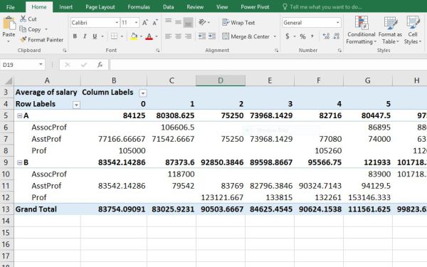
You will notice that after dragging the “salary” field into VALUES AREA it changes to “Sum of salary”. It gives the sum of salary for all the rows in original data set that match with given row and column criteria in Pivot Table. If there are five Assistant Professors in discipline “A” who has 10 years of service, it gives the sum of salary of the Assistant Professors in that category.
Let us say that we need to display the average salary instead of sum of salaries for each value field.
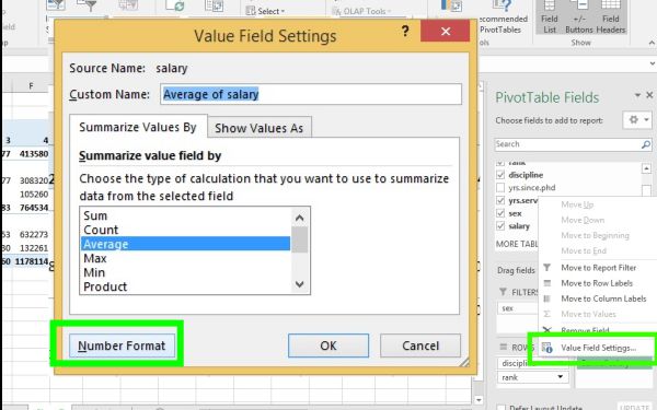
How to change value field settings in pivot table
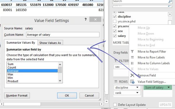
- Click the “sum of salary” item within the VALUES AREA
- Click “Value Field settings…” menu item from the menu popped up.
“Value Field Settings” dialog box will be appeared. - Select “Summarize Values By” tab
- Select “Average” from the selected field.
- Click OK.
Now you have completed the setting up of your basic Pivot Table. This table summarizes the average salary of each category of professors with different years of service.
How to group columns in pivot table
You can group the columns or rows of Pivot Tables. Grouping is a very useful feature. We will discuss about grouping in a different tutorial in detail.
For the time being, let us group the years of service columns into class intervals of 5 years. In this example we use automatic grouping option. This option works only on numerical or date fields only.
How to group items using automatic grouping option?
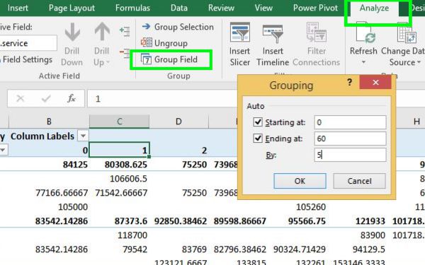
- Click one of the field items in years of service column labels.
- Go to “Analyze Tab” → “Group” command group → Click “Group Field”.
The “Grouping” dialog box appears. - Keep the “Starting at” and “Ending at” checked and default values unchanged. Make sure they represent the actual ends of the data series.
- Change the value of input box labeled as “By:” to 5.
- Click OK
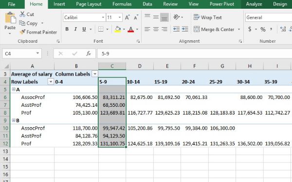
You will notice the columns of the table has been changed to represent class intervals of 5, in years of service.
ON and OFF displaying Sub totals and Grand totals
You can easily on or off sub totals and grand totals in a Pivot Table.
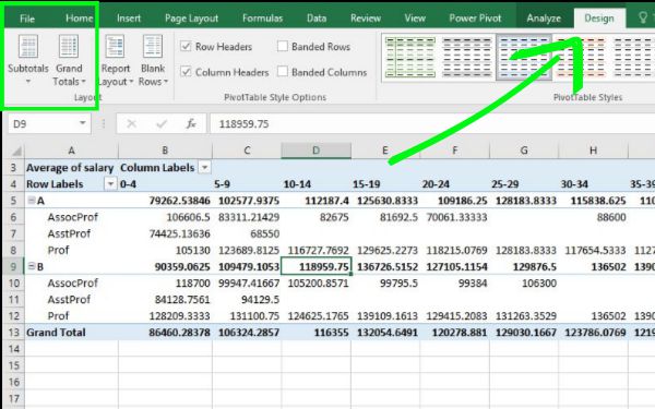
- Go to “PivotTable Tools” → “Design” → “Layout” command group.
- Click “Subtotals” → Select preferred option from the drop down menu. In this example let us click “Do Not Show Subtotals”
- Click “Grand Totals” → Select preferred option from the drop down menu. In this example let us click “Off for Rows and Columns”.
How to change pivot table style
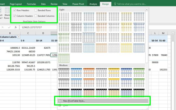
You can select any of the styles from the “PivotTable Styles” section of the “Design Tab”.
If you do not like any of the available styles, you can create a new Pivot Table Style.
You can also have the following options under “PivotTable Style Options”
• On and Off column and row headers.
• Apply or remove banded columns and rows to the Pivot Table.
How to change the number Formatting of Pivot Table Values
It will be very important to change the Number Format of the Pivot Table Values. You can follow the steps given below for that purpose.
- Click the relevant field item within the VALUES AREA of the Pivot Table Fields Task Pane. In this example, click on “sum of salary” item.
- Click “Value Field settings…” menu item from the menu popped up.
Value Field Settings dialog box will be appeared. - Click “Number Format” button.
- The usual “Format Cells” dialog box appears showing only the options for changing number formats in cells.
- Change the number format for Pivot Tables to suit the requirement.
In this example we have to use currency formats.
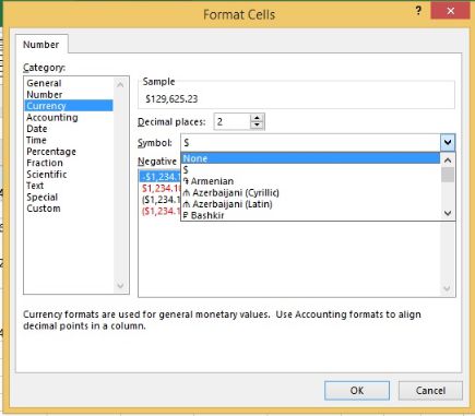
- Click “OK” after making the required adjustments to the number formatting.
Download the worked example file here.
SHARE