Regression analysis in Excel- Simply Explained [With Examples]

This tutorial created using Microsoft Excel 2019. Other compatible versions are Excel for Office 365 Excel for Office 365 for Mac; Excel 2016; Excel 2019 for Mac; Excel 2013; Excel 2010; Excel 2007; Excel 2016 for Mac; Excel for Mac 2011. If you find any issues doing regression analysis in those versions, please leave a comment below.

In this tutorial, we discuss how to do a regression analysis in Excel. I will teach you how to activate the regression analysis feature, what are the functions and methods we can use to do a regression analysis in Excel and most importantly, how to interpret the regression analysis results.

I will discuss following key topics on regression analysis using Excel. Also I have added worked example for you to study.

1. Manual method for simple linear regression analysis
2. Regression analysis with scatter plot charts with Trendline
3. Regression analysis with Excel formulas or worksheet functions
4. Detailed linear regression analysis in Excel using Analysis ToolPak
5. Interpretation of the regression analysis output in excel
6. Download the Regression analysis in Excel example file

Microsoft Excels functions and tools use the least squares method to calculate regression coefficients. Visit this useful article If you like to learn about least squares method before moving into regression analysis in excel.

Manual method of simple linear regression analysis with least squares method

You have to know at least a little bit about the regression formulas to carry out a manual regression analysis.

In simple linear regression, there is an independent variable (X) and a dependent variable (Y).

We assume that there is a linear relationship between the independent variable , X and the dependent variable , Y. Then we formulate the equation for that linear relationship between X and Y using regression theory.

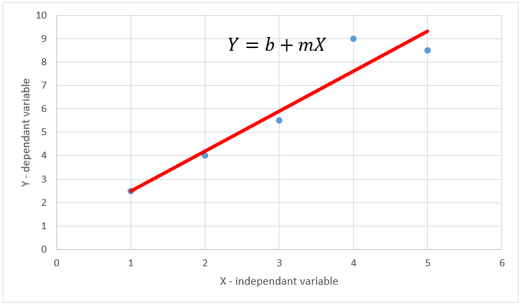
Regression equation,

Y = b + mX

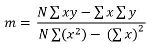
Equation for slope of the regression line,

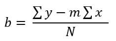
Equation for intercept of the regression line

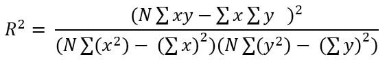
Equation for R-squared

Let us see an example to learn the procedure for regression analysis.

This regression model finds the relationship between advertising expenses and sales volume.

Regression analysis procedure in manual method

Step 01: set up the calculation table as follows. Keep columns for x,y, x², y² and xy.

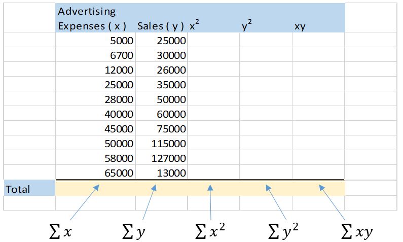
Step 02: Fill the table with respective x², y² and xy values.
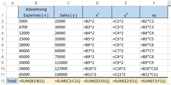
For calculation of x², y² and xy you can enter the formulas into first row. Then copy the formulas to other rows by dragging the fill handle. After that, get the sum of each column to the bottom row.

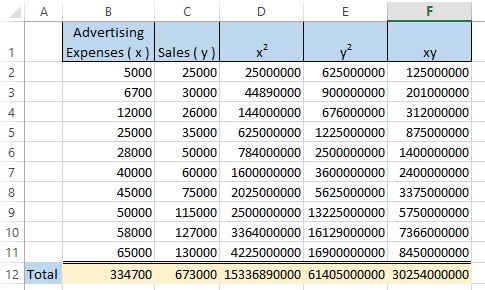
Finally your table should look like this.

Step 03: Calculate the regression coefficients using equations as follows.

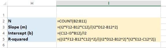
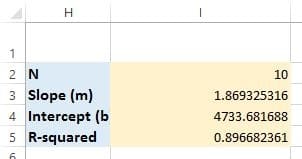
Now you should get your output as follows,

Interpretation of results of regression analysis in manual method.

Slope of the regression line (m) = 1.8693
Intercept of the regression line (b) = 4733.681
Therefore, the regression equation for this case is,

Y = 4733.681 + 1.8693X

We got an R-squared value equals to 0.896. It is very close to 1.0. That means there is a strong relationship between advertisement expenses (x) and the sales volume (y).

Regression analysis in excel using scatter plot charts with Trendline

You can use Microsoft Excel scatter charts when you want to do a quick and brief regression analysis. This method also uses the least squares method. In addition to simple linear regression, Trendline gives you the option to fit your data in to other regression models such as, exponential; logarithmic; polynomial; power and moving average.

Regression analysis procedure in excel using trendline option

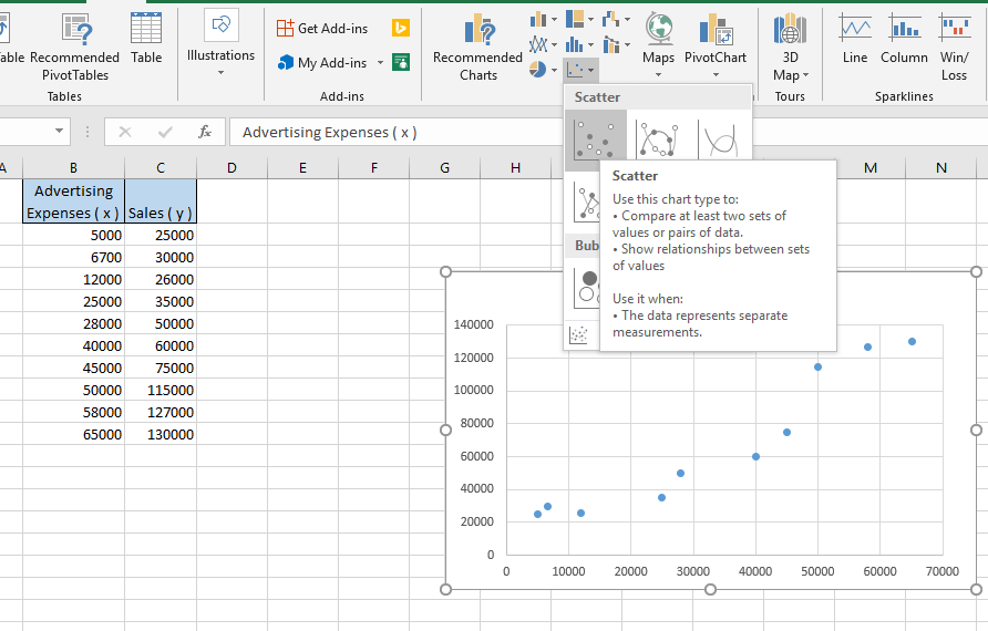
Step 01: Prepare your data in two adjacent columns. Make sure that your independent variable, x is in first column and the dependent variable, y is in next column.

Step 02 : Select both columns having X and Y values. You have the option to select with or without column headers.

Step 03: Go to → “Insert” Tab → “Charts” group → click “Insert scatter (X,Y ) or Bubble chart” button.
Select any of the Scatter Chart type provided in the drop menu. I prefer the first chart type having only points.

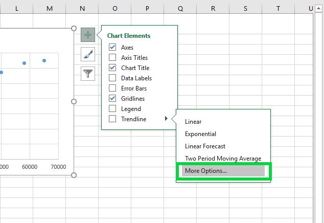
Step 04 : Click anywhere on the scatter chart. Three buttons will appear top right corner just outside the chart area.

Step 05 : Click the “Chart Elements” button which looks like thick ‘+’ symbol.

Step 06 : Move the mouse pointer on to the “Trendline” item of the appeared drop down menu.

Step 07 : Click the small black right-arrow head which appears in “Trendline” menu item.

Step 08 : Click “More options” menu item.

Now you will see that the “Format Trendline” pane appears right side of the Microsoft Excel window.
Step 09: Configure the trendline options as follows.

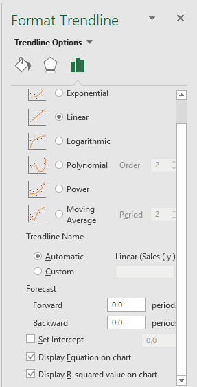
1) Select radio button for “Linear”.
2) Select the checkbox for “Display Equation on chart”.
3) Select the checkbox for “Display R – squared value on chart”.
Now, you can see the regression equation and R² value above the trendline.
Compare the equation to the equation we got in manual method. You should see that they are similar.

Regression analysis in Excel using formulas or worksheet functions

There are times that you only need to find regression coefficients. In that case you can simply use Excel worksheet functions or formulas. SLOPE (), INTERCEPT () and RSQ () are the main worksheet function you will need to find linear regression coefficients.
Prepare your independent (X) and dependent (Y) variable values as in previous cases.

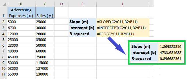
Calculate the slope of the regression line

Step 01 : Insert “= SLOPE ()” formula within a desired cell.
Step 02 : For the first parameter, select the Excel cell range that you have entered the Y-values which is the dependent variable. And for the second parameter select the cell range that you have entered the X-values which is the independent variable.
Step 03 : Press “Enter”.
Now we got the value for the slope of the regression line.

Calculate the intercept of the regression line

Step 01 : Insert “= INTERCEPT ()” formula within a desired cell.

Step 02 : Select the suitable the x and y ranges same as above SLOPE formula.

Step 03 : Press “Enter”.
Now we got the value for the intercept of the regression line.

Calculate the R-squared value of the regression model

Step 01 : Insert “= RSQ ()” formula within a desired cell.

Step 02 : Select the suitable the x and y ranges same as above SLOPE formula.

Step 03 : Press “Enter”
Now we got the value for the R-squared value of the regression line.
Compare the these coefficients to the coefficients we got in other two method. It is clear that they are similar.

Detailed linear regression analysis in Excel using Analysis ToolPak

The best method to do a detailed regression analysis in Excel is to use the “Regression” tool which comes with Microsoft Excel Analysis ToolPak. It is a very powerful add-in in Microsoft Excel. If you do not know anything about Analysis ToolPak, please go through this link to learn more.
First you should prepare your data as in previous cases.

Step 01: Go to → “Data tab” → “Analysis” group → click “Data Analysis” command button.

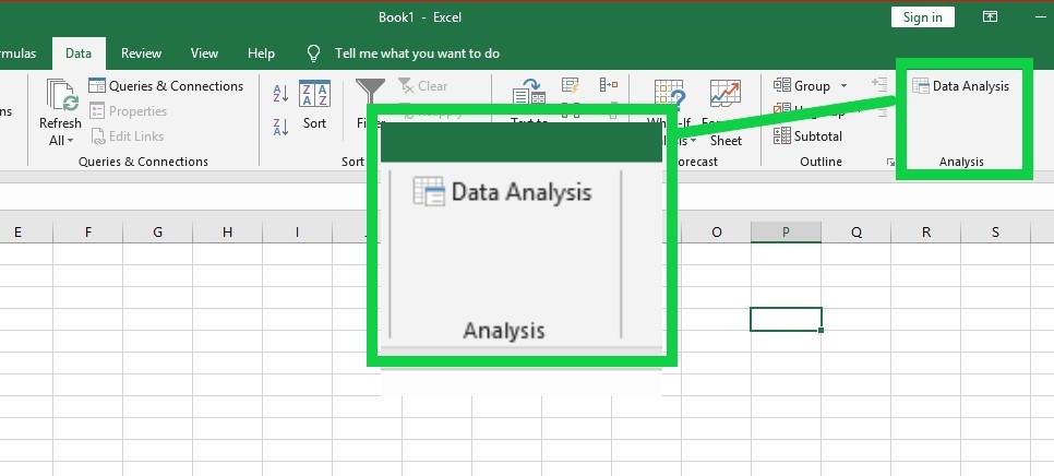
Now the “Data analysis” dialog box appears.
If you cannot find the “Data Analysis” button, go through the Analysis ToolPak tutorial here.

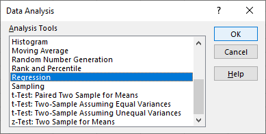
Step 02 : Select “Regression” from “Analysis Tools” list, then click “OK”.
Then the “Regression” dialog box appears.

Step 03: Configure the options for Regression analysis in “Regression” dialog box.

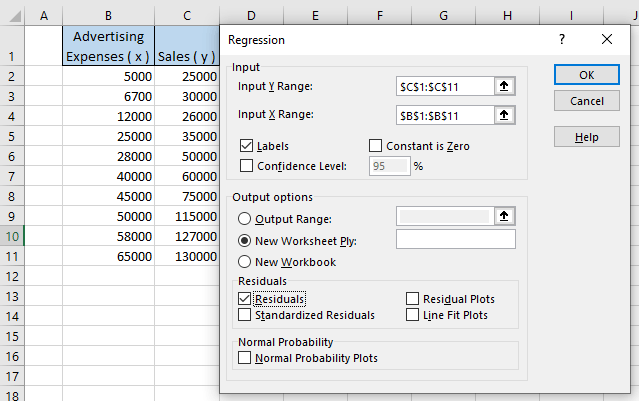
1. Select the cell range that contains your dependent variable for “input Y range”. Then select the cell range that contains your independent variable for “input X range”.
   If you need to do a multiple regression model use the following procedure. Arrange all the independent variables such that they are in adjacent columns. Select the whole range that contains independent variables as the “Input X range”.
2. Select the check box called “Label” if you selected the x and y ranges with their column headers or title.
3. Keep the default “Output options” selection as “New Worksheet Ply”.
4. Select “Residuals” options from “Residuals” group.
5. Click “OK”.

A new worksheet loads with the information for the regression analysis we just carried out in excel.

Interpretation of the regression analysis output in excel

Let us discuss the most important parts of information in the regression analysis output.

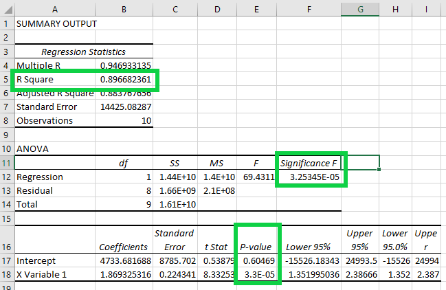
R – Squared

This is also called as the coefficient of determination. R-squared value indicates the strength of relationship between independent and dependent variable. A value that is closer to one indicates a stronger relationship. R-squared value that is closer to zero indicates a weaker relationship between dependent and independent variable.

Significance F

If the “significance F” value is lower than the significance level you consider which is 0.05 here, then your regression model is significant. That means it provides a better fit than the intercept only model. In statistics terms, you can reject the null hypothesis that the “regression model and intercept only model is equal”.

p-value for coefficients

The p-value located next to t-stat tells us the significance of each regression coefficient.
If it is lesser than 5% (0.05) you can conclude that it provides a better fit. When you get a higher p-value than the level of significance, the coefficients are not that good. Then you should carefully consider whether to include that coefficients in the final regression model or not.

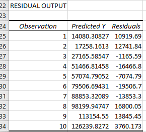
Residual output

Residual output shows the difference between the values predicted by regression model and observed values for dependent variable. You can get an overall assessment about how well your model behaves from the residual output.

Download the Regression analysis in Excel example file

You can download the excel file which has all the examples I have discussed above.