Most useful Excel Tips

Excel Tip #1 – Screen Scroll with arrow keys in excel while scroll lock on

If you press the arrow keys while in excel worksheet it changes the active cell based on the arrow key direction you are pressing. Sometimes it will be handy to scroll the screen using keyboard while keeping the active cell unchanged.
What you have to do is very simple to activate this scroll mode.

• There is a key called “Scroll lock” in the standard keyboard. In the laptop keyboards this key might be provided as a secondary function key along with a main key such as “Num lock”.

• Activate the scroll lock by pressing the “Scroll Lock” key or “fn” + “Scr lk” keys depending on the keyboard. You will be able to see a status bar note at bottom left corner of the window that it has activated the “Scroll Lock” mode.
• Now you can scroll the worksheet screen using arrow keys.
• Scroll the screen using key board arrow key without changing the active cell.

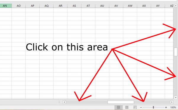
Excel Tip #2 – Scroll a complete screen in excel at once

Click either side of the scroll bar within the scroll box area. It will scroll the worksheet by one screen height or width.

Excel Tip #3 – Scroll with mouse wheel

You might already be using mouse wheel to scroll up or down the windows.
If you click the mouse wheel and move your mouse up or down it also scrolls the screen. Scroll speed increase or decrease with the distance you move the mouse.

Excel Tip #4 – zoom excel worksheet using mouse wheel

Press “Ctrl” button and then rotate the mouse wheel to zoom in or zoom out worksheet.

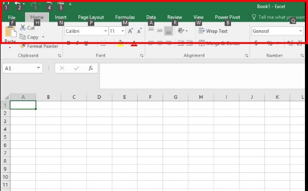
Excel Tip #5 – Show and Hide the Ribbon in excel

Ribbon is the area located top of the window with set of icons categorized under different tabs. This feature is available since Office 2007. The Ribbon in excel can be either hidden or visible.

Even if the Ribbon is hidden when you click on the Tab heading it becomes visible. Then it stays visible until you click anywhere outside the Ribbon Area.

There are three main methods to toggle the visibility of the Ribbon.

• Method 01: Press “Ctrl” + “F1” key
• Method 02: Double click a tab heading at the top
• Method 03: Right click the Ribbon area. A menu pops up. Click on the “Collapse the Ribbon” menu item.

Want to know how to build a soccer prediction app in excel? Read More here!

Excel Tip #6 – Keyboard shortcut to access Excel Ribbon commands

Ribbon supports keystroke to invoke commands. What you have to do is just press the “Alt” key which shows you the relevant “key tips”.
After that you just need to press the relevant keys for your command. No need to press “shift” key or “caps lock” or anything.

Imagine if you want to Protect the worksheet only using keystrokes. Protect sheet command is located within the “Review” tab.

• Step 01: Press “Alt” key which shows the “key tips”.
• Step 02: Type the keystroke belongs to the “Review” tab which “R”. It shows Ribbon for “Review” tab with relevant “key tips” for each command under review tab.
• Step 03: Type the keystroke combination belongs to the “Protect Sheet” command which is “PS”.

Excel Tip #7 – Repeat the last executed command in Excel

Imagine a situation where you want to apply the last command which you applied to one cell. You do not have to carry out same lengthy procedure again.

• Select the cell you want to apply the command.
• Press “Ctrl” + “Y” or “Ctrl” + “F4” keys.

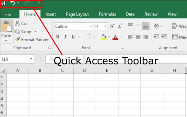
Excel Tip #8 – Use Quick Access toolbar to quickly access frequently used commands in excel

The quick access toolbar is very handy feature provided in the Excel to access frequently used commands quickly.

Quick access toolbar is located at top left corner of the Excel window.
Default setup gives the buttons to “Save”, “Undo” and “Redo” commands within the quick access toolbar.

You can easily customize the quick access tool bar to add more command buttons.

1. Click the down arrow head located right side of the Quick access toolbar.
2. A menu appeared with showing the commands you can add as quick access toolbar buttons.
3. You can click any of these items to select them to add to quick access toolbar.
4. If you are not satisfied with the given commands within the menu, there is another option to add “More commands”
5. Click “More command…” from “Customize Quick Access Toolbar” menu.
6. “Excel Options” dialog box appears showing all the commands you can add to the “Quick Access tool bar”.

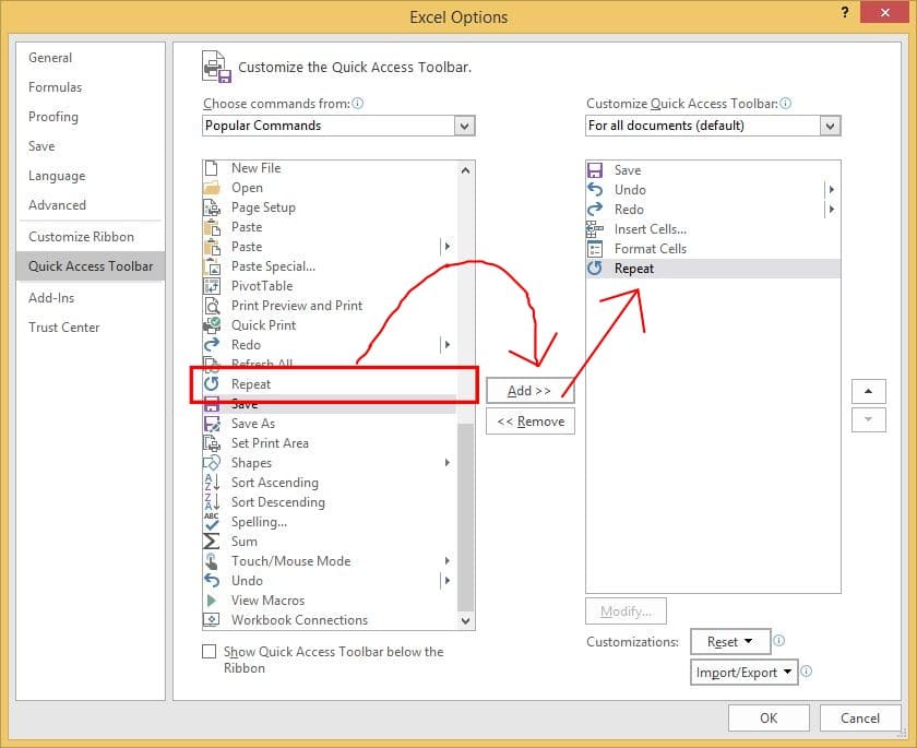
7. Select the command that you want to the add to the “Quick Access Toolbar” from the list in left side
8. Then click “Add >>” button
9. You can customize the quick access toolbar making it applicable to only the current work book or for all the documents you work with.
10. Select your preferred option from the “Customize Quick Access Toolbar” drop down menu.
11. Now click “OK”.

Excel Tip # 9 – Use fill handle auto fill data instantly in Excel

If you are going to fill a range of cells with data with some sort of pattern you do not have to fill them all manually in excel. Excel itself may be capable of doing it for you with its “Fill Handle” feature with minimum work.

Actually “Fill Handle” is a very sophisticated feature which deserves separate tutorial. But here I will explain basic usage with examples.

Example 01: Suppose that you want have a column filled with Months in the form of “Jan, Feb, March, …, Dec”.

• Step 1: Type “Jan” inside the first cell.
• Step 2: select the cell with “Jan”.

When you select a cell, excel marks the boundary of that cell with a thick green outline. There is small square located at bottom-right corner of the selected cell. We call it as the “Fill Handle”.

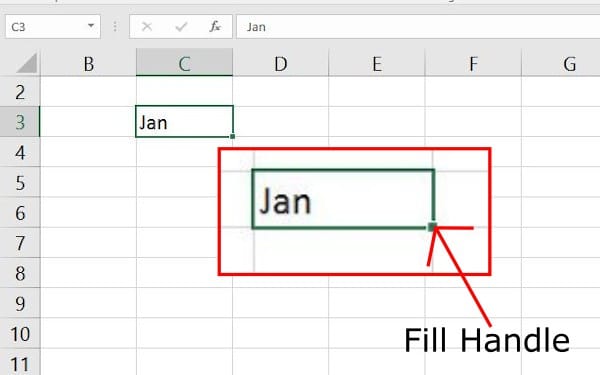
• Step 3: Move the cursor on to the fill handle until the cursor become a smaller cross hair. Then Click and drag the fill handle 11 rows down. You see that Excel automatically fills the Month names for you.

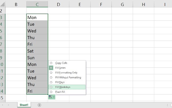
Example 02: Fill handle to insert a range with only weekdays in the form of “Mon, Tue, Wed, Thu, Fri, Mon, Tue, Wed, …,”

• Step 1: Type “Mon” inside the first cell.
• Step 2: select the cell with “Mon”.
• Step 3: Move the cursor on to the fill handle until the cursor become a smaller cross hair. Then Click and drag the fill handle around 14 rows down.

You see that Excel automatically fills the days of week for you. But only one issue is there that Excel has included weekends also. What to do about that?.
You can see a small icon has appeared near the bottom left corner of the data range you just created. That is call “Auto Fill Options” button.

• Step 4: Click the Auto Fill Options button.

Auto Fill Options menu appeared with few options you can select. In this case we want to fill the cells only weekdays.

• Step 5: Select “Weekdays” option.

Auto Fill Options menu shows you the options based on the type of series you are working with. So experiment with different type of data series like 1/5/2020,2/5/2020, …etc.

Auto fill text patterns combined with number

You can use auto fill handle to fill text based series with a number like Item 01, Item 02, Item 03, …
Just follow the same procedure as above.

Auto fill custom patterns

If you have to fill data with a custom pattern you have to let the excel identify that pattern. Therefore, you have to enter at least first two, three items of the series. Then select the all cells having the pattern. Now use fill handle to drag and complete the remaining cells with custom pattern.

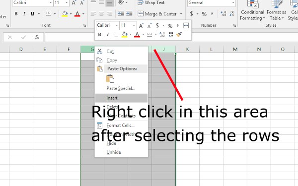
Excel Tip #10 – Quickly Insert new rows and columns to excel sheet

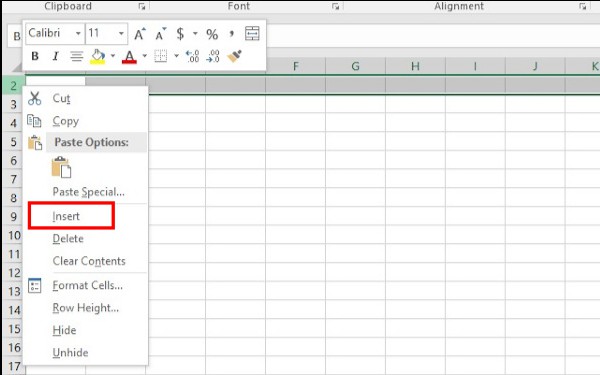
Inserting one row or column

• Right click the Row number or column number where you want to insert the new row or column.
• Select “Insert” from the appeared Shortcut Menu.

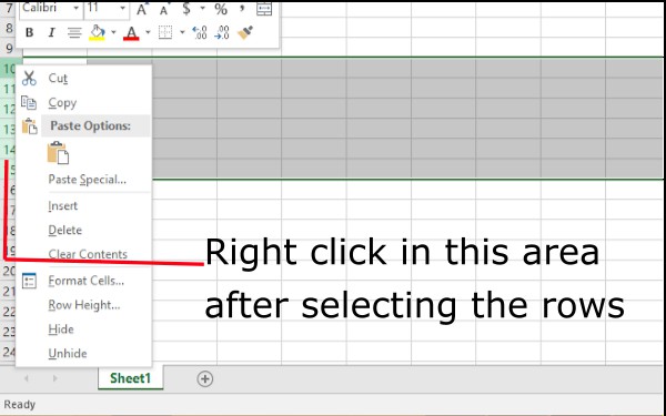
Insert multiple rows or columns

• Move the mouse cursor on to the row number or column number where you would like to insert new rows or columns.
• Click on the row number and drag down to select as many rows as you need to insert.

If it is the columns that you need to insert, then;

• Click on the column letter and drag left to select as many columns as you need to insert.
• Right Click on a row number or column letter within the selection.
• Now select “Insert” from the appeared Shortcut Menu.

Alternative method;

• Select the required number of rows or columns as mentioned above,
• Go to “Home” Tab → “Cells” command group → Click “insert” command button

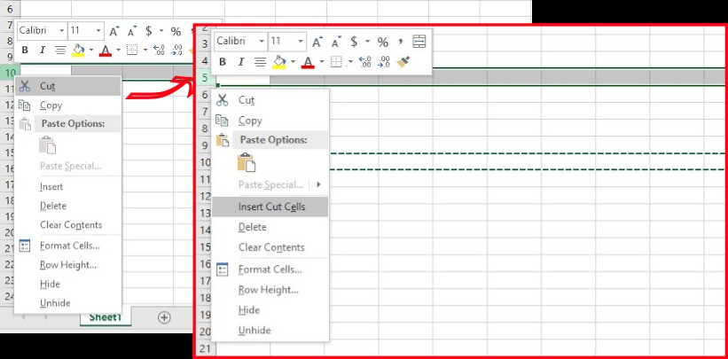
Excel Tip #11 – Move a Row or Column to different location in excel

Sometimes we need to move row or column in excel to different location.

• Click on the row number or column letter belongs to the respective row or column that you intend to move to select it.
• Then Right click on the row number or column letter.
• Select “Cut” from the appeared shortcut menu or press “Ctrl” + “X” keys.
• Then move the cursor on to the row number or column letter that you are going to insert the moved row or column.
• Right Click and Select “insert Cut Cells” from the appeared Shortcut Menu.

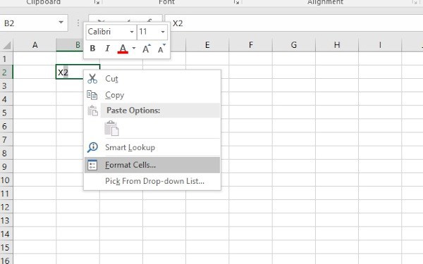
Excel Tip #12 – Subscript or superscript letters in excel

Sometimes we need to subscript or superscript letters entered within a cell.
One such occasion is when you enter squared notations like “X²”

• Enter the full text including the letter you want to superscript or subscript.
• Select the part of the text that you want superscript or subscript. Here we have to select “2” in the above text. If you are already selected another cell, you should double click the cell with the text to activate the cell text edit mode.

• Right click within the cell, then select “Format Cells…” from the appeared Shortcut Menu.

• “Format Cells” dialog box appears.
• Select the checkbox for “Superscript” or “Subscript” from the “Effects Group”

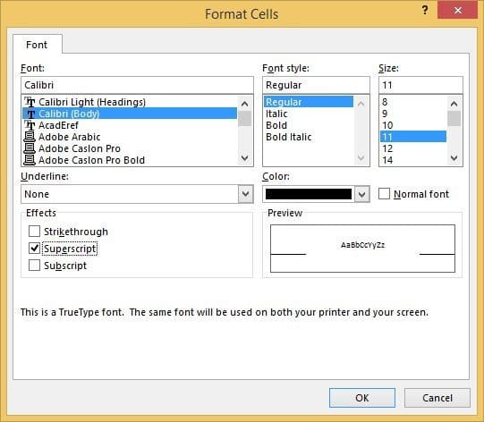
• Click “OK”.

Tip #13 – Add a line break to a text within a cell in excel

Usually text that typed within a cell appeared as single line. If the text length is longer than the column width it virtually overflows the cell boundary from the right side, if the right side cell is empty. Otherwise overflowing text part become invisible.

We can usually use “Wrap Text” command to overcome this issue as shown below.
Select Cell with the text. Then,

Go to “Home” tab → “Alignment” Command group → Click “Wrap Text”

What if you need enter a new line of text within the cell in excel?

• When you are at the end of the current line, Press “Alt” + “Enter”

If you want add new line of text to previously text entered cell,

• Activate the “Cell Edit Mode” by double clicking the cell.
• Move cursor to end of the current line text.
• Then Press “Alt” + “Enter”

Excel Tip #14 – Resize the Column Width or Row Height in excel to fit the content

More often than not, you would want to resize the column width to fit the content length. And sometimes it needs to resize the row height also.
If you want resize the column width in excel,

• Move the mouse cursor on to the right side boundary of the column within the “Column Letters” Area.
• Cursor changes to a “Slider” symbol, then double click column boundary.
• Column width resizes automatically to fit the longest content within cells of that column.
• If you want to resize the row height,
• Move the mouse cursor on to the lower boundary of the row within the “Row Number” Area.
• Cursor changes to a “Slider” symbol, then double click the row boundary.
• Row height resizes automatically to fit the longest content within cells of that column.

Excel Tip #15 – Merge Cells in Excel

Sometimes you want to combine or merge multiple cells to fit content in excel. This very common in table layouts you prepare within the Excel.

There are three different “Cell Merging” options provided within the Excel.

1. Merge and Center – This options merges the cells in to single larger cell and then center-align the content.
2. Merge Across – This option is very useful to merge cells in a selection across each row. It merges selected cells in same row to a single cell.
3. Merge Cells – This options merges the cells in to single larger cell.

So if you want to merge cells,

• Select the cells that you want to combine together
• Go to “Home” tab → “Alignment” Command group → Click “Merge and Center”

If you want different cells merging option,

• Click the down arrow head next to “Merge and Center” to pick how to merge cells.

You can also “unmerge” the merged cells in excel,

• Select the Merged cell that you want to unmerge.
• Go to “Home” tab → “Alignment” Command group → Click down arrow next to “Merge and Center”
• Select “Unmerge cells”

Things to remember when using Merge Cells!

• Merged cell gets the cell address of the top left corner cell.
• If you merge a range of cells, only the content within the top-left corner cell will be remained. If it is a single row or column, the content within the first cells will be remained.
• If you unmerge a merged cell with content, that content will be placed within the top left corner cell of the unmerged cell range.

Want to know how to create a drop down menu in excel? Read More Here!