Hazen-Williams Head Loss in Excel (Free Calculator, SI + US)
SHARE
Hazen-Williams gives the friction head loss of water flowing full in a pipe from four things: flow, internal diameter, length and a roughness coefficient C. In SI units:
hf, L and d in metres · Q in m³/s · C from 150 (PVC) down to under 100 (old cast iron)
In Excel
=10.67*B6*B12^1.852/(B10^1.852*B13^4.8704)Example: 1,200 m of 150 mm cement-lined ductile iron (C = 140) carrying 20 L/s loses 9.98 m of head, or 97.9 kPa.
Try the calculator below, download the finished workbook, or scroll down to build it yourself in SI or US units.
Hazen-Williams head loss calculator
Enter flow, internal diameter, length and pipe material to get head loss, pressure loss and velocity. Uses the same formulas as the Excel workbook: SI on the Calculator sheet, NFPA 13 on US units.
The Hazen-Williams formula in Excel
Hazen-Williams estimates the friction loss of water flowing full in a straight pipe. Allen Hazen and Gardner Williams fitted it to test data and published it in their Hydraulic Tables (1905). It is still the standard formula for water distribution design and fire sprinkler calculations. Engineers like it because it is explicit: you type it in and get an answer, with no friction factor to iterate.
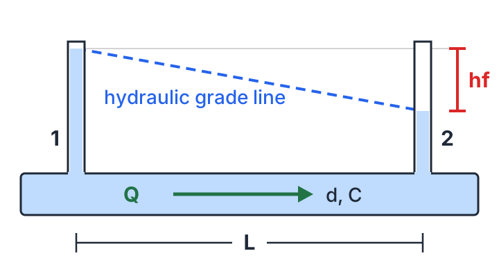
The two forms you will meet:
| Form | Formula | Units |
|---|---|---|
| SI | hf = 10.67 · L · Q^1.852 / (C^1.852 · d^4.8704) | hf, L, d in m; Q in m³/s |
| US (NFPA 13) | p = 4.52 · Q^1.85 / (C^1.85 · d^4.87) | p in psi per foot; Q in gpm; d in inches |
- C is the roughness coefficient: higher means smoother. PVC is 150, old cast iron can be below 100.
- 1.852 and 4.8704 are fitted exponents, not physics. Head loss grows with flow to the power 1.852, so doubling the flow multiplies the loss by about 3.6.
- d is the internal diameter, not the nominal size. A "150 mm" pipe's real ID can be 10 mm or more away from 150, depending on material and pressure class. Use the manufacturer's figure.
You will see slightly different constants in different references: 10.67 or 10.667, and d^4.87, d^4.8704 or d^4.871. They don't matter. For the example above they give 9.969 m (10.67 with 4.87), 9.977 m (10.67 with 4.8704) and 9.985 m (EPANET's 10.667 with 4.871). The NFPA form in US units gives 9.95 m. All four agree within 0.4%. EPANET, the US EPA's network model, uses the same formula internally (4.727 in feet and cfs, which converts to 10.667 in SI).
What does matter is C. That's further down.
Build the calculator step by step
The finished sheet has inputs in rows 4 to 10 and results in rows 12 to 19. Inputs are in the practical units engineers use (L/s, mm). The formula itself needs m³/s and m, so you convert first.
1. Enter the inputs. In Calculator, type the flow in B4 (L/s), the internal diameter in
B5 (mm) and the length in B6 (m). Put the material in B7. The workbook has 11 materials
on a C values sheet.
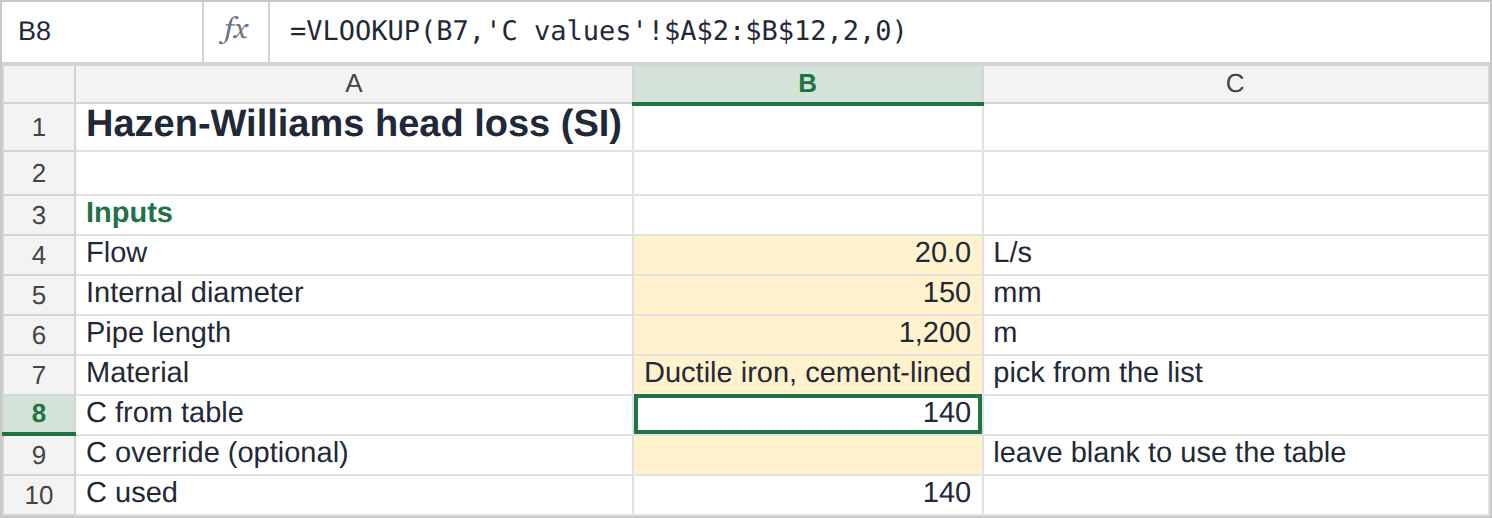
2. Look up C, with an override. Make B7 a dropdown (Data > Data Validation > List, source
='C values'!$A$2:$A$12; see drop-down lists in Excel).
Then pull its C value:
B8:  =VLOOKUP(B7,'C values'!$A$2:$B$12,2,0)
B10: =IF(B9="",B8,B9)
The 0 at the end asks for an exact match, the same as FALSE.
B9 is an optional override. Type a C value there when your utility or code says to use a
different one, and B10 uses it instead of the table.
3. Convert units. B12 is =B4/1000 (L/s to m³/s), and B13 is =B5/1000 (mm to m).
4. Head loss. This is the Hazen-Williams formula with the cell references:
B14: =10.67*B6*B12^1.852/(B10^1.852*B13^4.8704)
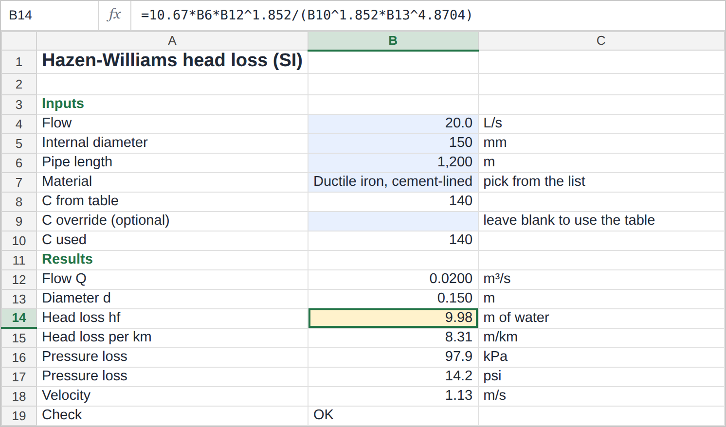
5. Turn it into numbers people use.
B15: =B14/B6*1000       head loss per km (m/km)
B16: =B14*9.81          pressure loss (kPa)
B17: =B14*1.4223        pressure loss (psi)
B18: =B12/(PI()*B13^2/4)  velocity (m/s)
6. Add a velocity check. Hazen-Williams is least reliable at very low and very high velocities (see When Hazen-Williams goes wrong), so flag them:
B19: =IF(B18<0.3,"Slow: HW underestimates loss",IF(B18>3,"Fast: check surge, use Darcy","OK"))
With 20 L/s in a 150 mm pipe the velocity is 1.13 m/s and the check says OK.
Hazen-Williams in US units (gpm, inches, psi)
Fire sprinkler, plumbing and irrigation designers in the US use the NFPA 13 form, which gives
pressure loss in psi per foot directly. The US units sheet has it, with an elevation term so
you get the pressure left at the far end:
B11: =4.52*B4^1.85/(B7^1.85*B5^4.87)     friction loss, psi per ft
B12: =B11*B6                             friction loss, psi
B14: =B8*0.4335                          elevation loss, psi (0.4335 psi per ft of water)
B15: =B9-B12-B14                         residual pressure, psi
B16: =B4*0.002228/(PI()*(B5/12)^2/4)     velocity, ft/s
The example is a 3/4" type L copper line (0.785 in ID), 100 ft long, C = 130, carrying 6 gpm up 15 ft from a 60 psi supply. Friction takes 5.0 psi (0.0496 psi/ft), the 15 ft rise takes 6.5 psi, and 48.5 psi is left at the fixture. Velocity is 3.98 ft/s, under the 5 ft/s often used as a limit to avoid noise and water hammer.
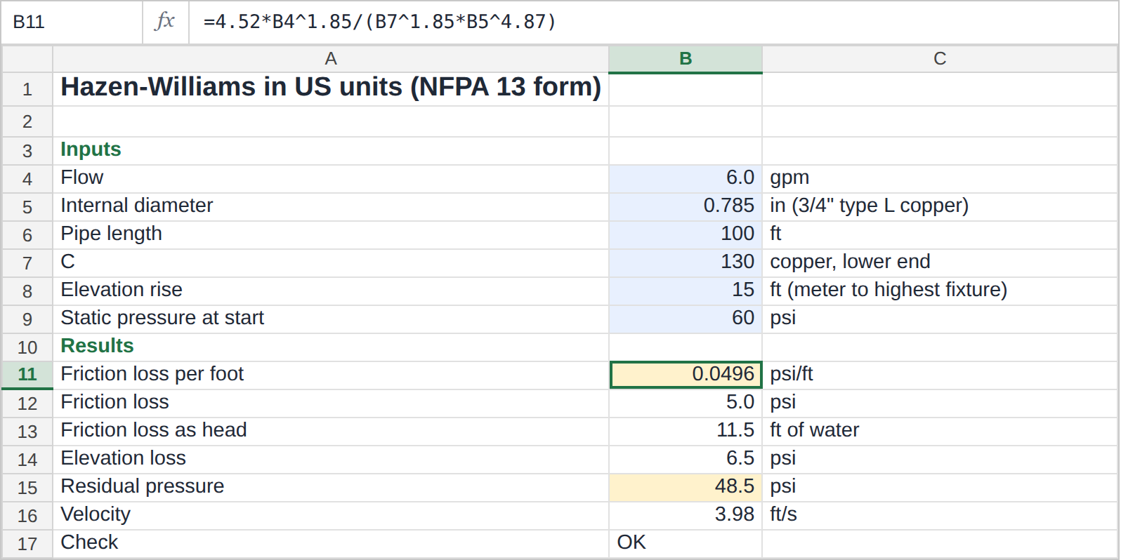
Rows 20 to 26 run the SI example through the NFPA formula as a check: 317.0 gpm in a 5.906 in pipe over 3,937 ft loses 14.16 psi, which is 9.95 m against 9.98 m from the SI sheet, a 0.2% difference.
If you're a homeowner trying to work out why the shower is weak, start with what normal house water pressure is. For irrigation zones, see how to work out sprinkler design capacity and working pressure.
Solve for flow or diameter
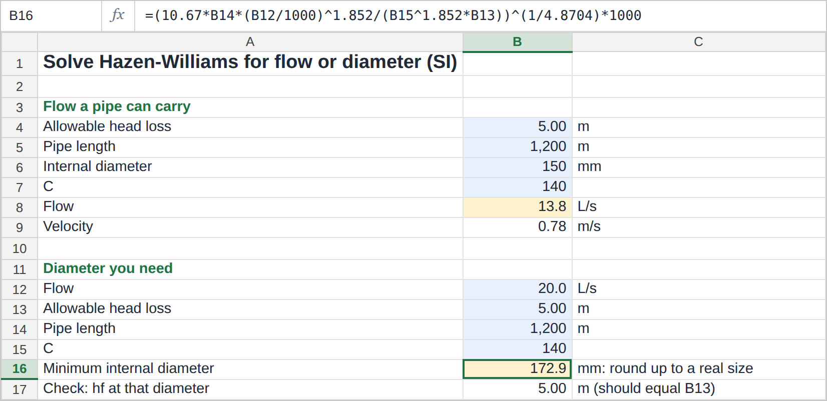
Hazen-Williams rearranges cleanly, so you don't need Goal Seek. The Solve for sheet has both.
How much flow can this pipe carry for an allowable head loss B4 (m), length B5, ID B6 (mm) and C B7:
B8: =(B4*B7^1.852*(B6/1000)^4.8704/(10.67*B5))^(1/1.852)*1000
A 150 mm pipe, 1,200 m long with C = 140, can carry 13.8 L/s if you allow 5 m of loss (velocity 0.78 m/s).
What diameter do I need for flow B12 (L/s), allowable loss B13, length B14 and C B15:
B16: =(10.67*B14*(B12/1000)^1.852/(B15^1.852*B13))^(1/4.8704)*1000
To carry 20 L/s over 1,200 m with no more than 5 m of loss you need 172.9 mm internal
diameter. Round up to the next pipe you can actually buy, then check its real ID back in the
calculator. B17 puts the answer back into the head loss formula and returns 5.00 m, which
confirms the rearrangement.
Worked example: pipes in series
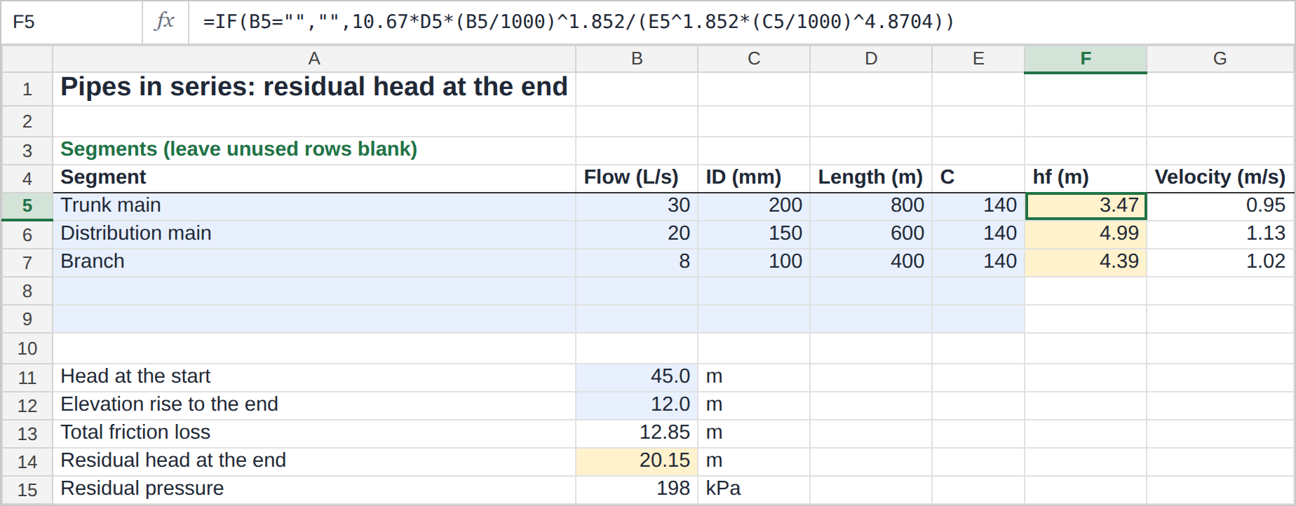
Real systems are several pipes end to end. The Pipe run sheet takes up to five segments, works
out the head loss of each with the same formula, and subtracts the total and the elevation rise
from the head at the start:
F5:  =IF(B5="","",10.67*D5*(B5/1000)^1.852/(E5^1.852*(C5/1000)^4.8704))
B14: =B11-B12-B13
The example is a trunk main, a distribution main and a branch, all C = 140:
| Segment | Flow (L/s) | ID (mm) | Length (m) | hf (m) | Velocity (m/s) |
|---|---|---|---|---|---|
| Trunk main | 30 | 200 | 800 | 3.47 | 0.95 |
| Distribution main | 20 | 150 | 600 | 4.99 | 1.13 |
| Branch | 8 | 100 | 400 | 4.39 | 1.02 |
Total friction is 12.85 m. Starting from 45 m of head with a 12 m rise, 20.15 m (198 kPa) is left at the end of the branch. Notice that the shortest pipe is not the one with the smallest loss: the 100 mm branch loses more per metre than the trunk main.
This example is a typical design case, not a specific network. To see how the result reacts to
flow, put B14 in a one-variable data table, or vary
flow and diameter together with a two-variable data table.
Choosing the C value
This is where the answer really moves. Rows 22 to 25 of the Calculator sheet rerun the
150 mm example at other C values:
| C | Head loss (m) | vs C = 140 |
|---|---|---|
| 150 | 8.78 | −12% |
| 140 | 9.98 | (base) |
| 130 | 11.44 | +15% |
| 110 | 15.59 | +56% |
| 100 | 18.60 | +86% |
Ten points of C is a 12-15% change, far more than any difference between published constants. Old pipe makes it worse. Unlined cast iron drops from about 130 new to 107-113 after 10 years and 89-100 after 20 as the bore scales and tubercles grow. If you design a rehabilitation with the new-pipe C, you underestimate the loss badly: at C = 100 the same pipe loses 18.60 m, not 11.44 m.
Typical values (in the workbook's C values sheet):
| Material | C |
|---|---|
| PVC | 150 |
| Polyethylene (PE/HDPE) | 140 |
| Ductile iron, cement-lined | 140 |
| Asbestos-cement | 140 |
| Copper | 130-140 |
| Cast iron, new / 10 yr / 20 yr | 130 / 107-113 / 89-100 |
| Concrete | 100-140 |
| Steel | 90-120 |
| Galvanized iron | 120 |
Use your utility's design standard or the code's table where one applies. NFPA 13, for example, fixes C for sprinkler pipe by material and system type. For an existing main you can back-calculate C from a field test (two pressure readings and a measured flow) with the same rearrangement as the flow formula above.
When Hazen-Williams goes wrong
Hazen-Williams has no viscosity and no Reynolds number in it, so it is only as good as the range
it was fitted on: water at ordinary temperatures (roughly 4-25 °C, 40-75 °F) in turbulent flow,
at velocities around 1 m/s. To see how far it drifts outside that range, the HW vs Darcy sheet
compares it with Darcy-Weisbach for PVC (C = 150, roughness 0.0015 mm), water at 20 °C:
| ID (mm) | 0.3 m/s | 1 m/s | 2 m/s | 3 m/s |
|---|---|---|---|---|
| 20 | −21% | −8% | −3% | 0% |
| 50 | −12% | −2% | +2% | +4% |
| 100 | −7% | +2% | +5% | +7% |
| 200 | −3% | +4% | +7% | +8% |
| 500 | +1% | +6% | +8% | +8% |
Positive means Hazen-Williams gives more loss than Darcy-Weisbach. (The Darcy friction factor here comes from the Swamee-Jain approximation, which is within about 1% of Colebrook.)
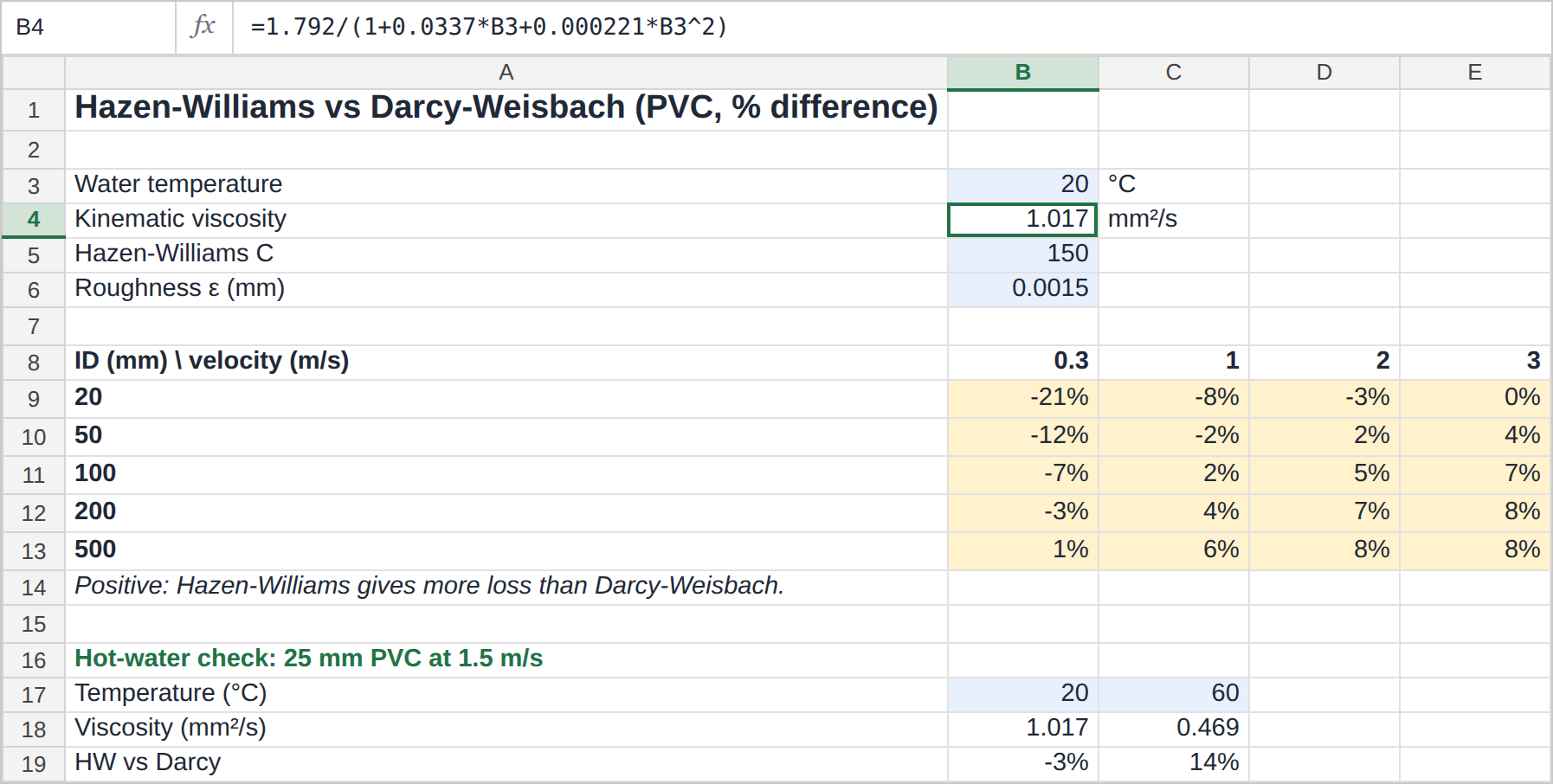
What the grid shows:
- Small, slow pipes: Hazen-Williams underestimates. A 20 mm pipe at 0.3 m/s comes out 21% low. Low flow in small pipes is the least turbulent case, where a fixed C fits worst.
- Large, fast pipes: it overestimates by 6-8%. That's on the safe side for design, which is part of why it's accepted for mains.
- Hot water: it can't tell. In the hot-water check (rows 17 to 19), a 25 mm pipe at 1.5 m/s goes from −3% at 20 °C to +14% at 60 °C, because hot water is less than half as viscous and Darcy-Weisbach sees that. Use Darcy-Weisbach for hot water lines.
- Not water: don't use it. Oil, glycol mixes, slurries and gases all need Darcy-Weisbach.
- Fittings aren't included. Hazen-Williams covers the straight pipe. Add bends, valves and meters as equivalent lengths or K values on top.
Excel errors you are likely to hit:
#VALUE!when an input holds text, for example "150 mm" typed intoB5. Keep units in their own column.#DIV/0!from a zero diameter or C, and#NUM!from a negative one (a negative number can't be raised to a fractional power).- A head loss that is off by a factor of thousands or more usually means mm or L/s went into the
formula without being converted (
B12,B13). #N/AinB8when the material inB7doesn't exactly match a row of theC valuessheet.
Optional: a reusable HAZEN function with LAMBDA
In Excel 365 (and Excel 2024) you can turn the formula into your own function. Go to Formulas >
Name Manager > New, name it HW_HEADLOSS, and in Refers to paste:
=LAMBDA(L,Q,C,d, 10.67*L*Q^1.852/(C^1.852*d^4.8704))
Then =HW_HEADLOSS(B6,B12,B10,B13) anywhere in the workbook returns the same 9.98 m. LAMBDA
isn't available in Excel 2021 and older. There, use a
VBA function or an add-in instead: see custom functions and add-ins in Excel.
The download doesn't need it: it uses plain formulas.
FAQ
What is the Hazen-Williams C value for PVC?
150 for new PVC. Some designers use 140 to allow for ageing and joints. Polyethylene is usually 140.
Is the Hazen-Williams equation accurate?
For water at normal temperatures in pipes from about 50 to 500 mm at 1-3 m/s, it is within about ±8% of Darcy-Weisbach (see the grid above). It gets worse in small pipes at low velocity and in hot water. In practice the uncertainty in C is usually bigger than the formula's own error.
Hazen-Williams vs Darcy-Weisbach: which should I use?
Hazen-Williams for cold-water distribution, irrigation and fire sprinklers, where it's the industry and code standard and C values are well known. Darcy-Weisbach for anything else: hot water, other fluids, very small or very smooth pipes, laminar flow.
Can you use Hazen-Williams for hot water?
Not reliably. It has no viscosity term, so in the workbook's check it is 14% off at 60 °C in a 25 mm pipe. Use Darcy-Weisbach with the viscosity at the actual temperature.
What does 1.852 mean in the Hazen-Williams formula?
It is the flow exponent Hazen and Williams fitted to their test data. Head loss rises with flow to the power 1.852, so 10% more flow means about 19% more loss. The NFPA form rounds it to 1.85.
Download the workbook
Download hazen-williams-excel.xlsx. Plain formulas, no macros, works in Excel 2016 and later, Excel for Mac and LibreOffice. Input cells are shaded blue.
| Sheet | What it does |
|---|---|
Calculator |
SI head loss from flow (L/s), diameter (mm), length and material, plus pressure loss, velocity check, C sensitivity and constant comparison |
US units |
NFPA 13 form in gpm, inches and psi, with elevation and residual pressure, and the SI cross-check |
Solve for |
Flow a pipe can carry, and the diameter you need, for an allowable head loss |
Pipe run |
Up to five pipes in series, total loss and residual head at the end |
C values |
Hazen-Williams C for 11 pipe materials, used by the dropdown |
HW vs Darcy |
Percentage difference from Darcy-Weisbach by diameter, velocity and water temperature |
The calculator at the top of this page uses the same SI formula and gives the same 9.98 m for the worked example.
Sources: Williams, G.S. and Hazen, A., Hydraulic Tables, John Wiley & Sons (1905; later editions
to 1920). Rossman, L.A., EPANET 2 Users Manual, US EPA, EPA/600/R-00/057 (2000), and the
EPANET source code (src/hydcoeffs.c). NFPA 13,
Standard for the Installation of Sprinkler Systems, hydraulic calculation procedures. C values
from Wikipedia's Hazen-Williams article,
which compiles standard tables.
SHARE